import numpy as np
import torch
from torch import nn
The Simplest Autoencoder
Last updated: Jan 26, 2025.
The backpropagation algorithm for training neural networks seemed very complicated when I first encountered it. I only really understood it after implementing it from scratch following the excellent video by Andrej Karpathy (2022). It also helped me to realize that backpropagation is a kind of automatic differentiation (AD) and can be understood without any reference to neural networks. See (Baydin et al. 2015) for an excellent survey of AD in machine learning.
After understanding backprop, though, I had a different question: why did it take so long to discover and become popular? The story of that seems surprisingly complicated but a good starting point is the blog post by Liu (2023).
While reading through that post a couple of quotes from Geoffrey Hinton caught my eye:
So they just refused to work on [backprop], not even to write a program, so I had to do it myself.
I almost blew it because the first thing I tried it on was an 8-3-8 encoder; that is, you have eight input units, three hidden units, and eight output units. You want to turn on one of the input units and get the same output unit to be on.
I went off and I spent a weekend. I wrote a LISP program to do it.
I love learning about the history of computing so in this post we’ll try to recreate what Hinton must have done in that weekend.
The neural network he’s describing (“8-3-8”) is an autoencoder, whose job is to learn to simply reproduce its output as faithfully as it can. This might seem pointless, but it makes more sense when you think of the network as containing both an encoder and a decoder along with a “bottleneck” in the middle where the input vector gets squashed to one with a lower dimension. This squashing can be variously understood as a lossy compression of the input, as dimensionality reduction, or as feature extraction. For our purposes here though, it’s just a toy historical example demonstrating the value of backpropagation.
The input dataset for our network are the numbers \(1\) - \(8\) encoded as “one-hot” vectors.
\[ \begin{aligned} 1 = [0 0 0 0 0 0 0 1] \\ 2 = [0 0 0 0 0 0 1 0] \\ ... \\ 8 = [1 0 0 0 0 0 0 0] \end{aligned} \]
Thus the input layer and output layers both have size \(8\), and we’ll introduce a hidden layer inbetween of size \(3\), hence giving the network the name “8-3-8” encoder. The hidden layer is of size \(3\) because \(3\) bits is all you need to represent eight unique values. The network and the learning algorithm are described in detail in (Rumelhart, Hinton, and Williams 1986, chap. 8) though the terminology is a little archaic.
8-3-8 in PyTorch
Let’s implement the autoencoder using PyTorch.
The eight inputs together can be represented as an 8x8 matrix.
INPUTS = torch.diag(torch.ones(8))
INPUTS
tensor([[1., 0., 0., 0., 0., 0., 0., 0.],
[0., 1., 0., 0., 0., 0., 0., 0.],
[0., 0., 1., 0., 0., 0., 0., 0.],
[0., 0., 0., 1., 0., 0., 0., 0.],
[0., 0., 0., 0., 1., 0., 0., 0.],
[0., 0., 0., 0., 0., 1., 0., 0.],
[0., 0., 0., 0., 0., 0., 1., 0.],
[0., 0., 0., 0., 0., 0., 0., 1.]])The network is a Sequential stack, which means the inputs only flow forward (“feed-forward”). We’ll use the sigmoid as the activation for historical accuracy.
from collections import OrderedDict

class AutoEncoder(nn.Module):
    def __init__(self):
        super().__init__()
        self.stack = nn.Sequential(OrderedDict([
            ('hidden', nn.Linear(8, 3, bias=True)),
            ('output', nn.Linear(3, 8, bias=True)),
            ('sigmoid', nn.Sigmoid())
        ]))

    def forward(self, x):
        return self.stack(x)
The network can be visually shown as:

We need to pick a loss function before training the network. Given that the input and output are one-hot vectors, this could be seen as a classification task and thus the cross-entropy loss function is suitable. Using cross-entropy indeed works very well, but we’ll use the mean-squared loss instead to stay true to the historical paper.
A couple of other notes on the training:
We’ll use the entire set of 8 inputs in every batch.
My first attempt at the training code didn’t work and I spent a lot of time tinkering with the loss function and the hyperparameters before someone pointed out that PyTorch doesn’t reset the gradient values automatically. Adding the line
sgd.zero_grad()fixed the problem.
Thanks to Prakhar Dixit for pointing out the above mistake.
def train(epochs: int, lr: float, momentum: float):
    model = AutoEncoder()

    loss_fn = nn.MSELoss(reduction='mean')
    sgd = torch.optim.SGD(model.parameters(), lr=lr, momentum=momentum)

    prev_loss = 1e9
    loss = 0
    losses = []

    for i in range(epochs):
        x = INPUTS
        yhat = model(x)
        prev_loss = loss
        loss = loss_fn(yhat, x)

        sgd.zero_grad()
        loss.backward()
        sgd.step()

        if i % 5000 == 0:
            print(f"i = {i:6}, loss: {loss:>7f}")

        losses.append(loss.item())

    return model, losses
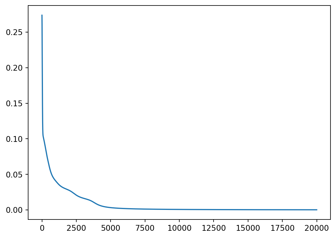
We can now run the training and plot the loss curve.
import matplotlib.pyplot as plt

torch.manual_seed(42)
net, losses = train(20000, 0.1, 0.9)
plt.plot(range(len(losses)), losses)
i = 0, loss: 0.273701
i = 5000, loss: 0.003292
i = 10000, loss: 0.000732
i = 15000, loss: 0.000383
We can see that the network has learnt to very closely match the inputs by printing the result of running all 8 inputs through it.
torch.set_printoptions(linewidth=120, sci_mode=False)
net(INPUTS)
tensor([[ 0.9644, 0.0000, 0.0000, 0.0000, 0.0087, 0.0000, 0.0000, 0.0099],
[ 0.0087, 0.9795, 0.0143, 0.0000, 0.0000, 0.0000, 0.0000, 0.0128],
[ 0.0002, 0.0232, 0.9732, 0.0079, 0.0000, 0.0215, 0.0000, 0.0000],
[ 0.0012, 0.0010, 0.0301, 0.9525, 0.0286, 0.0077, 0.0152, 0.0191],
[ 0.0407, 0.0000, 0.0000, 0.0185, 0.9771, 0.0000, 0.0198, 0.0002],
[ 0.0001, 0.0000, 0.0139, 0.0000, 0.0000, 0.9795, 0.0162, 0.0000],
[ 0.0040, 0.0000, 0.0000, 0.0000, 0.0123, 0.0156, 0.9793, 0.0000],
[ 0.0397, 0.0208, 0.0000, 0.0153, 0.0002, 0.0000, 0.0000, 0.9763]],
grad_fn=<SigmoidBackward0>)